What is SMARTASS?

SMARTASS is intended to be used by institutional and educational companies and organizations with the aim of efficiently assigning their employees and members on the basis of several criteria such as distance, cost or CO2 emission. It uses several parameters such as energy unit cost (gas, electricity etc. or ZERO cost energy), CO2 emission per unit of distance or ZERO CO2 emission.

The assignment can be of two types:

• by hand (manual)
• optimal (automatically)

In both cases, depending on the enterprise goals the result may be given by a matrix of 3 kinds :

• distance matrix
• cost matrix
• CO2 matrix

Moreover, SMARTASS presents resulting assignments and summaries in a dynamic fashion and in many forms:

• User assignment matrix (by hand)
• Optimal assignment matrix
• Comaprison and savings summary between user-hand and optimal assignments
• Graphic representation of different comparison matrices
• Map routes corresponding to the optimal or user matrix
• The BEST choice between the 3 possible goals (optimize distance, cost or CO2)

In the sequal, speaking about cost matrix may have one of three significance "distance cost", "money matrix"="cost matrix" or "CO2 matrix".

For which purpose SMARTASS could be used?

SMARTASS can be used :

• By any company to assign its employees to their clients in order to optimize travel costs and minimize the carbon footprint
• By any institutional organization (education, social, political etc.) to minimize travel cost of their members and employees

This version is limited to associate only one contact to each address with respect to a departure or destination point.

How to call SMARTASS from your WEB site ?

SMARTASS may be used directly or by calling it programmatically from any WEB page in a very simple way as summarized below:

In both cases (MAPS or WEATHER call) you access to all features of SMARTASS application.

SMARTASS standard flowchart

Global flowchart

SMARTASS flowchart is simple and illustrated in the following image:

Hand vs Optimal assignment flowchart

Assignments goals and the BEST choice flowchart

How to use SMARTASS?

Define general options

General options apply to all created objects, if they are not defined at their creation time. Options are related to projects in such a way each project has its own options that apply to all created objects belonging to the project (departure/destination points, contacts etc. ). The following options are avaialable:

• Distance unit: Can be fixed to KM (Kilometer), M (Meter) or Mile
  
  
• Energy cost per distance unit: This option determines the travel cost depending on the distance between two points A (Departure) and B (Destination). Travel cost depends on contact's unit energy cost if they use travel mode consumming gas, electricity or any kind of energy.
  
  
• Used currency:choose your local or any country currency to be used in all calculations and outputs. Selected currency is used in all total costs as well as unit costs.
  
  
• CO2 emission per distance unit (g/dist. Unit): Based on this option we calculate the total CO2 emission for a travel between two points A and B. Note that by default this parameter is expressed in gramme by unit of distance. For example if the contact vehicule is 110 g/KM CO2 emission, then we suppose that the distance unit is KM, otherwise you have to evaluate this parameter in terms of g/Dist. unit as 110 g/KM is equivalent to 68,73 g/MILE if the chosen distance unit is MILE.

Add Markers

We can add markers in three ways:

• local address: In this case, you have to activate geolocation in your navigator. Some navigators require HTTPS site like GOOGLE CHROME in which case this option will not work correctly.
  
  
• Specific address: type your address which can be a town or a complete or partial address (number, street, town, country).
  
  
• Specific (latitude, longitude): type latitude and longitude values varying respectively between -86 and 86, -180 and 180. Note that not in all cases the corresponding address is resolved.
  
  

Once the marker option is chosen, we can add it as a "Departure point" or as "Destination point" by clicking on the appropriate button:

• +A: to add a "Departure point"
• +B: to add a "Destination point"

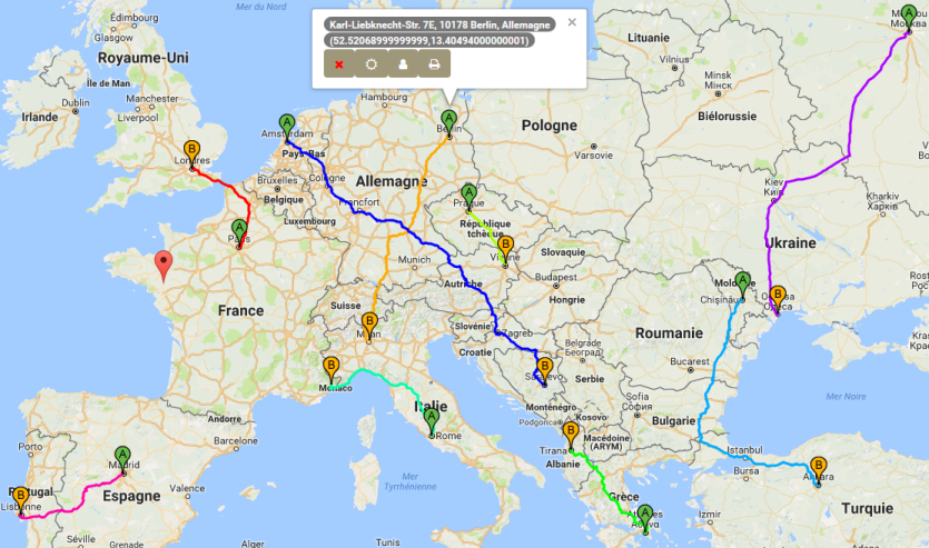
Markers can be moved around the map and related data are automatically updated to reflect the new address. At any time only one marker representing departure or destination point, is the current address. A simple click on the marker, make it as the current address and update its data if necessary. We can from the info-window associated with a marker, delete, show address's meteo, edit the associated contact or simply print the map.

Manage Departure and Destination Points

"Departure Points" and "Destination Points" are formed of rows. Each row represents a point with these data:

• Address: Geographic Point address
  
  
• Latitude: Address latitude
  
  
• Longitude: Address longitude
  
  
• Associated contact: Associated Contact details to the point (First Name, Last Name, EMAIL etc.). If the contact is associated to a destination point, all related travel properties are not used as energy cost, CO2 emission and travel mode.

"Departure points" and "Destination points" are organized in two matrices where each matrix record has the following fields:

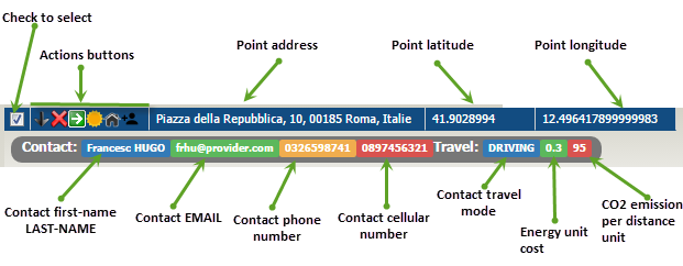
Each a "Departure point" or a "Destination point" may have some actions summarized as follows (All actions are under the grids field named "Actions"):

Associate contacts to points

People are associated to points (A or B). As said before, we can associate only one contact to any point. In order to associate more than one contact to a point, we can make a duplicate point to which associate the second contact and so on. Default travel mode, Energy cost and CO2 emission are significant only for contacts associated to departure points. These values if not fixed for a contact, they will take default values defined in project options.

Each contact has the following fields:

• Contact type: can be
  • "Enterprise contact" (as B point to which we could assign A point contact)
  • "Employee" associated to A point
  • "Student" associated to A point
  • "Others" any other contact type to associate to A or B point
    
    
• First Name
  
  
• Last Name
  
  
• EMAIL
  
  
• Phone number
  
  
• Cellular phone number
  
  
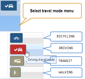
• Default travel mode: 4 travel modes are available (BICYCLING, DRIVING, TRANSIT and WALKING)
  
  
• Gas cost per distance unit: This can be fixed for all contacts in general options or defined for each contact depending on the chosen travel mode and the contact engine if DRIVING is used.
  
  
• CO2 emission per distance unit: This data is necessary to compute Total CO2 emission related to the assignment computed matrix.

Build Matrices

There are 3 kinds of matrices, each is related to the optimisation nature (Distance, Cost or CO2). For each type, you can make your own assignments (by hand) or compute automatically the optimal matrix and then compare between hand-assignment and optimal-assignment matrices. At this step you are able to generate 3 types of matrices as illustrated in the following image and sections below: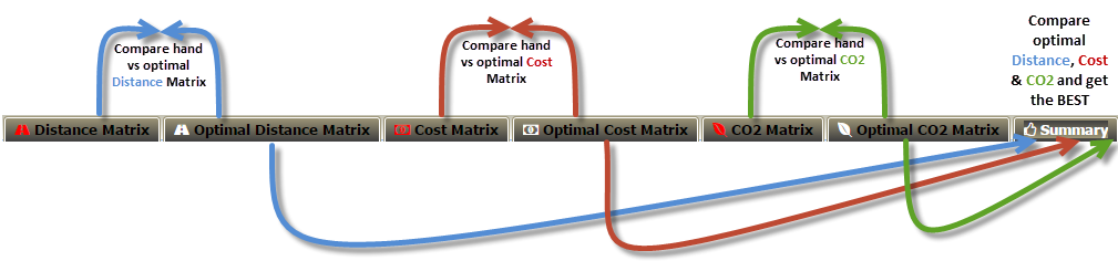

Distance matrices

• Manual matrix: Activate Distance matrix tab, then for each departure point check only one entry corresponding to the destination point. The summary matrix is generated dynamically on the top toolbar with selected entries number.
  
  
• Optimal matrix: the optimal distance matrix is generated automatically once you activate the corresponding tab Optimal Distance Matrix and resulting summary matrix is displayed on the top toolbar.

Cost matrices

Note that results and total cost related to the cost matrix are different from the distance matrix only if energy unit cost associated with contacts are not all identical. This happens when contacts have vehicles with different energy cost (Diesel, Gasoline etc.), even 0 energy cost in bicycling or walking cases.

• Manual matrix: Activate Cost matrix tab, then for each departure point check only one entry corresponding to the destination point. The summary matrix is generated dynamically on the top toolbar with selected entries number.
  
  
• Optimal matrix: the optimal cost matrix is generated automatically once you activate the corresponding tab Optimal Cost Matrix and resulting summary matrix is displayed on the top toolbar.

CO2 matrices

Note that results and total cost related to the cost matrix are different from the distance matrix only if energy unit cost associated with contacts are not all identical. This happens when contacts have vehicles with different energy cost (Diesel, Gasoline etc.), even 0 energy cost in bicycling or walking cases.

• Manual matrix: Activate CO2 matrix tab, then for each departure point check only one entry corresponding to the destination point. The summary matrix is generated dynamically on the top toolbar with selected entries number.
  
  
• Optimal matrix: the optimal CO2 matrix is generated automatically once you activate the corresponding tab Optimal Cost Matrix and resulting summary matrix is displayed on the top toolbar.

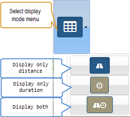
Matrices Display options

Only in distance matrix case as well as cost matrix and CO2 matrix the following input and display features are available and can be selected at any time:

• Travel mode: 4 travel modes are available (BICYCLING, DRIVING, TRANSIT and WALKING). Make sure that all contacts associated to departure points have the same chosen travel mode. If the chosen travel mode is not appropriate you may have errors in GOOGLE services response in the resulting matrix entries.
  
  
• Display type: You can choose between 3 types of display (only distance, only duration or both) in distance matrix case. What ever display mode you choose, it doesn't have any effect on the obtained results.

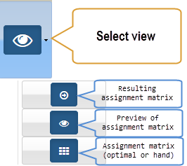
Get summary results

Many featured Results are given, summarized as follows:

• Resulting assignment matrix: This matrix displays chosen (or optimal) assignments (source and destination) with corresponding fields values (distance, duration, cost and CO2 emission) and totals for each of these fields.
  
  
• Assignment matrix preview: it represents resulting assignment matrix with focus on the chosen or optimal entries.
  
  
• Graphic assignment: it represents resulting assignment graphic with focus on the chosen or optimal entries.
  
  
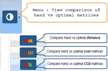
• Hand and optimal matrices comparison summary: it is given by a table displayed on the top tool bar in which are summarized hand assignment data, optimal data and realized savings between both in terms of distance, duration, cost and CO2 emission. See driven examples below for such a summary table.
  
  
• Distance, Cost and CO2 matrices comparison summary: it is given by a comparison summary table in which are summarized hand-assignment as well as optimal assignment results between distance, cost and CO2 emission. See driven examples below for such a summary table.

Matrices common toolbar

A dynamic common toolbar is present on the top of matrices dialog window as follows:

The following summaries common tools available on the common toolbar:

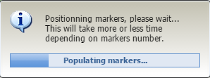
Icons and messages Indicators

As mentioned above, responses sent by GOOGLE services to queries are asynchronous. Therefore, a waiting time is required for each sent request. In order to be informed by the current processing, a graphic or textual status is displayed to the end-user. The following table summarizes the standby and status indicators:

Printing

Printing functionality is contextual and may have 2 goals:

• : Print current panel content.
  
  
• : Print a picture of the current panel as seen on the screen.
  
  

NOTE

In general, distance and cost optimal assignment matrices are different only if associated contacts have not the same "energy unit cost". Otherwise they are identical and total distance as well as total cost are obviously equal. On the other hand, distance and CO2 optimal assignment matrices are different only if associated contacts have not the same "CO2 unit cost". Choosing "optimal distance matrix" "optimal cost matrix" or "optimal CO2 matrix" depends on the institutions and enterprises goals:

• have the optimum total travel distance regardless of the total cost and CO2
• have the optimum total cost regardless of the total distance and CO2
• have the optimum total CO2 regardless of the total distance and cost

What ever the chosen strategy is, we can simulate all these scenarios, compare between the totals (distance, cost and CO2) and then we could choose the best one.

In general we have the following assertion:

To be more precise, we will present in the following sections 2 driven examples you can realize in SMARTASS application.

Driven examples (visit of European cities)

In all given examples we are organizing 9 trips from 9 to 9 European cities. This example is one of many working samples available in the application from menu Samples containing these samples :

Each of these samples represents a working project that can be saved locally on your local hard disk of your device and opened later from SMARTASS. All these operations are available in the SMARTASS top toolbar:

The "Project" button allows to open an existing project or create a new one as indicated in the following dialog:

The "options" button allows you to fix options for the current opened project as indicated in the following dialog:

The departure and destination points are defined as follows (expressed in French):

Departures Adresses	Destinations Adresses
Bill JOHNSON•bj@provider.com•0123654789•0632598741 Hôtel de Ville, 75004 Paris, France	7 Whitehall, London SW1A 2DD, Royaume-Uni
JOSIF YOUSEF•jyou@provider.fr•0236541789•0987456321 Karl-Liebknecht-Str. 7E, 10178 Berlin, Allemagne	Kulla e Sahatit, Tirana 1001, Albanie
Rudolph ANTONIO•rant@provider.com•0965321478•0789654123 Náměstí Míru 820/9, Vinohrady, 120 00 Praha-Praha 2, République tchèque	Labenbacher Weg, 1210 Wien, Autriche
Julien MICKAEL•jmic@provifer.fr•0365214789•0698745123 Pl. Omonias 19, Athina 105 52, Grèce	Route de la Vésubie, 06450 Utelle, France
Francesc HUGO•frhu@provider.com•0326598741•0897456321 Piazza della Repubblica, 10, 00185 Roma, Italie	E761, Bulozi, Bosnie-Herzégovine
Rolando ZENO•roz@providder.com•0321456987•0652314789 str. Haltei, Chișinău, Moldavie	Via Sant'Uguzzone, 8, 20126 Milano, Italie
Ede FABIANO•edf@provider.com•0985632147•0784596321 Oudezijds Achterburgwal 1921, 1012 DX Amsterdam, Pays-Bas	Torhova St, 33, Odesa, Odessa Oblast, Ukraine, 65000
Herbert WENDEL•hew@provider.com•0123654780•0621056879 pr-d Voskresenskiye Vorota, 1А, Moskva, Russie, 109012	Campo Mártires da Pátria 125, 1150 Lisboa, Portugal
Tarik MISSAD•tam@provider.com•0123654789•0698523477 Av. de Arqueros, 3, 28024 Madrid, Espagne	Anafartalar, A.Adnan Saygun Cd No:12, 06050 Altındağ/Ankara, Turquie

The purpose is that any contact from a departure capital should visit only one destination city such that :

• Case 1: total distance of all 9 trips is the minimum possible
• Case 2: total cost of all 9 trips is the minimum possible
• Case 3: total CO2 emission of all 9 trips is the minimum possible

Note that reported results below in terms of distance/cost/CO2 may be lightly different from those you will obtain, because Google services results depend on the traffic and other parameters at the time are obtained.

Driven example 1: Distance optimization

In this case, our objective is to to minimize total distance between departure and destination points such that each contact must visit only one European city. To achieve this, follow the steps below:

Step 1

To generate departure and destinaton points listed above, click on "Samples" and then choose "Visit European cities" as indicated in the image above. Note that markers are generated asynchronously and it will take some minutes for that depending on your Internet connection and used device.

Step 2

Optionnaly, you may fix options by clicking on the command button . In this example, we leave default options, namely:

• Distance unit: KM
• Energy cost by distance unit: 0.12
• Used currency: Euro Member-EUR (€)
• CO2 emission by distance unit: 92 g/KM

Since all our sample contacts associated to departure points have aleady energy cost and CO2 emission values, we do not have to change all options except if necessary "distance unit" or "used currency".

Step 3

Optionnaly, for each departure point change associate contact (First Name, Last Name etc.) as an example see the lists above. Click on + to add/change a contact to a point. All departure points contacts for our sample are aleady completed.

Step 4

Optionnaly if not already done, select by checking the top check box all departure and destination points (total of 9 addresses for each).

Step 5

Click on Distance Matrix command button to generate corresponding hand assignment matrix. Check for each departure point a corresponding and unique destination point (total of 9 assignments). CHECK EXACTLY 9 DIFFERENT ENTRIES WITH DIFFERENT DEPARTURE POINTS.

Step 6

Click on Optimal Distance Matrix to generate by the application corresponding optimal assignment matrix.

You should get the following summary table for the optimal distance matrix:

Travel mode	Distance	Duration	Cost	CO2
DRIVING	7878.29 KM	87h22min1sec	2648.8 €	589.87 KG

The resulting optimal distance assignment matrix must be the folllowing:

Contact Adresse	Assigned to	Distance	Duration	Cost	CO2
Bill JOHNSON•bj@provider.com•0123654789•0632598741• Hôtel de Ville, 75004 Paris, France	•••• Route de la Vésubie, 06450 Utelle, France	966.55 KM	8h56min44sec	289.97 €	82.16 KG
JOSIF YOUSEF •jyou@provider.fr•0236541789•0987456321• Karl-Liebknecht-Str. 7E, 10178 Berlin, Allemagne	•••• E761, Bulozi, Bosnie-Herzégovine	1409.64 KM	14h44min57sec	352.41 €	77.53 KG
Rudolph ANTONIO•rant@provider.com•0965321478•0789654123• Náměstí Míru 820/9, Vinohrady, 120 00 Praha-Praha 2, République tchèque	•••• Labenbacher Weg, 1210 Wien, Autriche	284.17 KM	3h35min7sec	93.78 €	29.84 KG
Julien MICKAEL•jmic@provifer.fr•0365214789•0698745123• Pl. Omonias 19, Athina 105 52, Grèce	•••• Kulla e Sahatit, Tirana 1001, Albanie	703.39 KM	9h31min40sec	133.64 €	77.37 KG
Francesc HUGO•frhu@provider.com•0326598741•0897456321• Piazza della Repubblica, 10, 00185 Roma, Italie	•••• Via Sant'Uguzzone, 8, 20126 Milano, Italie	579.87 KM	5h40min24sec	173.96 €	55.09 KG
Rolando ZENO•roz@providder.com•0321456987•0652314789• str. Haltei, Chișinău, Moldavie	•••• Anafartalar, A.Adnan Saygun Cd No:12, 06050 Altındağ/Ankara, Turquie	1445.46 KM	17h47min36sec	332.46 €	101.18 KG
Ede FABIANO•edf@provider.com•0985632147•0784596321• Oudezijds Achterburgwal 1921, 1012 DX Amsterdam, Pays-Bas	•••• 7 Whitehall, London SW1A 2DD, Royaume-Uni	540.21 KM	6h21min42sec	54.02 €	29.71 KG
Herbert WENDEL•hew@provider.com•0123654780•0621056879• pr-d Voskresenskiye Vorota, 1А, Moskva, Russie, 109012	•••• Torhova St, 33, Odesa, Odessa Oblast, Ukraine, 65000	1332.92 KM	15h16min6sec	879.73 €	59.98 KG
Tarik MISSAD•tam@provider.com•0123654789•0698523477• Av. de Arqueros, 3, 28024 Madrid, Espagne	•••• Campo Mártires da Pátria 125, 1150 Lisboa, Portugal	616.07 KM	5h27min45sec	338.84 €	77.01 KG
(DRIVING)	TOTAL:	7878.29 KM	87h22min1sec	2648.8 €	589.87 KG

The corresponding routes on the map are the following:

Step 7

In this step you will evaluate the savings between hand and optimal assignments. To see the summarized savings, click on the sub-menu:

• for distance matrix:
  
  

For the distance matrix case you should get a summary table like the following (the savings depend on the hand chosen matrix):

Mode	Entries type	N of Entries	Travel mode	Distance	Duration	Cost	CO2
OPTIMAL	DISTANCE	9	DRIVING	7878.29 KM	87h22min1sec	2648.8 €	589.87 KG
manual	DISTANCE	9	DRIVING	19516.34 KM	195h20min	7505.67 €	1.55 T
Your savings:				11638.05 KM	107h57min59sec	4856.87 €	963.78 KG
Saving %:				147.72 %	123.58 %	183.36 %	163.39 %

Step 8

In order to view graphically the comparison matrix between hand and optimal assignments, you click on the menu to have the following beautiful column graph:

To close the graph dialog, just click second time on the above button or the times button on the dialog itsef.

Driven example 2 : Cost optimization

In this case, our objective is to to minimize total cost between departure and destination points such that each contact must visit only one European city. You can already guess that the obtained minimum cost in this case should be better than the one of the distance minimization case. But what about total distance, total duration and total CO2 emission compared to the previous case? That's what we will discover below.

Go through the following steps exactly as the same as in the distance case except for matrices generation.

Step 1

This step is identical to step 1 in the distance optimization case.

Step 2

This step is identical to step 2 in the distance optimization case.

Step 3

This step is identical to step 3 in the distance optimization case.

Step 4

This step is identical to step 4 in the distance optimization case.

Step 5

Click on Cost Matrix command button to generate corresponding hand cost assignment matrix. Check for each departure point a corresponding and unique destination point (total of 9 assignments). CHECK EXACTLY 9 DIFFERENT ENTRIES WITH DIFFERENT DEPARTURE POINTS.

Step 6

Click on Optimal Cost Matrix to generate by the application corresponding optimal cost assignment matrix.

You should get the following summary table for the optimal cost matrix:

Travel mode	Distance	Duration	Cost	CO2
DRIVING	8369.54 KM	93h19min8sec	2575.67 €	608.41 KG

The resulting optimal cost assignment matrix must be the folllowing:

Contact Adresse	Assigned to	Distance	Duration	Cost	CO2
Bill JOHNSON•bj@provider.com•0123654789•0632598741• Hôtel de Ville, 75004 Paris, France	•••• 7 Whitehall, London SW1A 2DD, Royaume-Uni	469.34 KM	5h21min41sec	140.8 €	39.89 KG
JOSIF YOUSEF •jyou@provider.fr•0236541789•0987456321• Karl-Liebknecht-Str. 7E, 10178 Berlin, Allemagne	•••• Via Sant'Uguzzone, 8, 20126 Milano, Italie	1043.02 KM	10h20min36sec	260.75 €	57.37 KG
Rudolph ANTONIO•rant@provider.com•0965321478•0789654123• Náměstí Míru 820/9, Vinohrady, 120 00 Praha-Praha 2, République tchèque	•••• Labenbacher Weg, 1210 Wien, Autriche	284.17 KM	3h35min7sec	93.78 €	29.84 KG
Julien MICKAEL•jmic@provifer.fr•0365214789•0698745123• Pl. Omonias 19, Athina 105 52, Grèce	•••• Kulla e Sahatit, Tirana 1001, Albanie	703.39 KM	9h31min40sec	133.64 €	77.37 KG
Francesc HUGO•frhu@provider.com•0326598741•0897456321• Piazza della Repubblica, 10, 00185 Roma, Italie	•••• Route de la Vésubie, 06450 Utelle, France	740.75 KM	7h59min38sec	222.23 €	70.37 KG
Rolando ZENO•roz@providder.com•0321456987•0652314789• str. Haltei, Chișinău, Moldavie	•••• Anafartalar, A.Adnan Saygun Cd No:12, 06050 Altındağ/Ankara, Turquie	1445.46 KM	17h47min36sec	332.46 €	101.18 KG
Ede FABIANO•edf@provider.com•0985632147•0784596321• Oudezijds Achterburgwal 1921, 1012 DX Amsterdam, Pays-Bas	•••• E761, Bulozi, Bosnie-Herzégovine	1734.43 KM	17h58min59sec	173.44 €	95.39 KG
Herbert WENDEL•hew@provider.com•0123654780•0621056879• pr-d Voskresenskiye Vorota, 1А, Moskva, Russie, 109012	•••• Torhova St, 33, Odesa, Odessa Oblast, Ukraine, 65000	1332.92 KM	15h16min6sec	879.73 €	59.98 KG
Tarik MISSAD•tam@provider.com•0123654789•0698523477• Av. de Arqueros, 3, 28024 Madrid, Espagne	•••• Campo Mártires da Pátria 125, 1150 Lisboa, Portugal	616.07 KM	5h27min45sec	338.84 €	77.01 KG
(DRIVING)	TOTAL:	8369.54 KM	93h19min8sec	2575.67 €	608.41 KG

The corresponding routes on the map are the following (different from the distance matrix case):

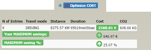
Step 7

In this step you will evaluate the savings between hand and optimal assignments. To see the summarized savings, click on the sub-menu:

• for cost matrix:

For the cost matrix case you should get a summary table like the following (the savings depend on the hand chosen matrix):

Mode	Entries type	N of Entries	Travel mode	Distance	Duration	Cost	CO2
OPTIMAL	COST	9	DRIVING	8369.54 KM	93h19min8sec	2575.67 €	608.41 KG
manual	COST	9	DRIVING	19516.34 KM	195h20min	7505.67 €	1.55 T
Your savings:				11146.79 KM	102h52sec	4930 €	945.25 KG
Saving %:				133.18 %	109.32 %	191.41 %	155.36 %

Step 8

In order to view graphically the comparison matrix between hand and optimal assignments, you click on the menu to have the following beautiful column graph:

Driven example 3 : CO2 optimization

In this case, our goal is to to minimize total CO2 between departure and destination points such that each contact must visit only one European city. You can already guess that the obtained minimum CO2 in this case should be better than the one of the distance minimization case as well as the cost minimization case. But what about total distance, total duration and total cost compared to the previous cases? That's what we will discover below.

Go through the following steps exactly as the same as in the previous cases 1 and 2, except for matrices generation.

Step 1

This step is identical to step 1 in the distance optimization case.

Step 2

This step is identical to step 2 in the distance optimization case.

Step 3

This step is identical to step 3 in the distance optimization case.

Step 4

This step is identical to step 4 in the distance optimization case.

Step 5

Click on CO2 Matrix command button to generate corresponding hand CO2 assignment matrix. Check for each departure point a corresponding and unique destination point (total of 9 assignments). CHECK EXACTLY 9 DIFFERENT ENTRIES WITH DIFFERENT DEPARTURE POINTS.

Step 6

Click on Optimal CO2 Matrix to generate by the application corresponding optimal CO2 assignment matrix.

You should get the following summary table for the optimal CO2 matrix:

Travel mode	Distance	Duration	Cost	CO2
DRIVING	7940.04 KM	92h12min44sec	3227.47 €	561.37 KG

The resulting optimal CO2 assignment matrix must be the folllowing:

Contact Adresse	Assigned to	Distance	Duration	Cost	CO2
Bill JOHNSON•bj@provider.com•0123654789•0632598741• Hôtel de Ville, 75004 Paris, France	•••• Route de la Vésubie, 06450 Utelle, France	966.55 KM	8h56min44sec	289.97 €	82.16 KG
JOSIF YOUSEF •jyou@provider.fr•0236541789•0987456321• Karl-Liebknecht-Str. 7E, 10178 Berlin, Allemagne	•••• E761, Bulozi, Bosnie-Herzégovine	1409.64 KM	14h44min57sec	352.41 €	77.53 KG
Rudolph ANTONIO•rant@provider.com•0965321478•0789654123• Náměstí Míru 820/9, Vinohrady, 120 00 Praha-Praha 2, République tchèque	•••• Labenbacher Weg, 1210 Wien, Autriche	284.17 KM	3h35min7sec	93.78 €	29.84 KG
Julien MICKAEL•jmic@provifer.fr•0365214789•0698745123• Pl. Omonias 19, Athina 105 52, Grèce	•••• Kulla e Sahatit, Tirana 1001, Albanie	703.39 KM	9h31min40sec	133.64 €	77.37 KG
Francesc HUGO•frhu@provider.com•0326598741•0897456321• Piazza della Repubblica, 10, 00185 Roma, Italie	•••• Via Sant'Uguzzone, 8, 20126 Milano, Italie	579.87 KM	5h40min24sec	173.96 €	55.09 KG
Rolando ZENO•roz@providder.com•0321456987•0652314789• str. Haltei, Chișinău, Moldavie	•••• Torhova St, 33, Odesa, Odessa Oblast, Ukraine, 65000	194.51 KM	3h2min38sec	44.74 €	13.62 KG
Ede FABIANO•edf@provider.com•0985632147•0784596321• Oudezijds Achterburgwal 1921, 1012 DX Amsterdam, Pays-Bas	•••• 7 Whitehall, London SW1A 2DD, Royaume-Uni	540.21 KM	6h21min42sec	54.02 €	29.71 KG
Herbert WENDEL•hew@provider.com•0123654780•0621056879• pr-d Voskresenskiye Vorota, 1А, Moskva, Russie, 109012	•••• Anafartalar, A.Adnan Saygun Cd No:12, 06050 Altındağ/Ankara, Turquie	2645.63 KM	34h51min47sec	1746.12 €	119.05 KG
Tarik MISSAD•tam@provider.com•0123654789•0698523477• Av. de Arqueros, 3, 28024 Madrid, Espagne	•••• Campo Mártires da Pátria 125, 1150 Lisboa, Portugal	616.07 KM	5h27min45sec	338.84 €	77.01 KG
(DRIVING)	TOTAL:	7940.04 KM	92h12min44sec	3227.47 €	561.37 KG

The corresponding routes on the map are the following (different from the distance matrix case):

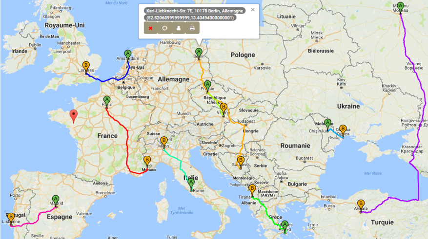
Step 7

In this step you will evaluate the savings between hand and optimal assignments. To see the summarized savings, click on the sub-menu:

• for cost matrix:

For the CO2 matrix case you should get a summary table like the following (the savings depend on the hand chosen matrix):

Mode	Entries type	N of Entries	Travel mode	Distance	Duration	Cost	CO2
OPTIMAL	CO2	9	DRIVING	7940.04 KM	92h12min44sec	3227.47 €	561.37 KG
manual	CO2	9	DRIVING	19516.34 KM	195h20min	7505.67 €	1.55 T
Your savings:				11576.3 KM	103h7min16sec	4278.2 €	992.28 KG
Saving %:				145.8 %	111.83 %	132.56 %	176.76 %

Step 8

In order to view graphically the comparison matrix between hand and optimal assignments, you click on the menu to have the following beautiful column graph:

SUMMARY: Compare distance/cost/CO2 optimal matrices and get THE BEST

In this section you will discover and generate summary elements (matrices, graphs etc.):

• SUMMARY MATRIX: Compares between the 3 optimal matrices (distance, cost and CO2) and gives maximum possible savings for each criterion.
  
  
• GRAPH: Compares graphically between the 3 optimal matrices (distance, cost and CO2). The generated colomn graph corresponds to the previous "SUMMARY MATRIX".
  
  
• WHAT IS YOUR GOAL? In this section, SMARTASS gives you the corresponding "SUMMARY MATRIX" depending on your goal. The resulting matrix simply represents an extraction of the previous global "SUMMARY MATRIX" depending on your chosen goal (Optimize distance, cost or CO2).
  
  
• WHAT IS THE BEST AMONG THE 3 GOALS? In this section, SMARTASS gives you the best optimal solution among the 3 goals (Optimize distance, cost or CO2). It may happen that all 3 goals are best as you can see through some given samples.

We discover all these sections applied to our driven example below:

SUMMARY MATRIX:

A summary matrix for optimal solutions (distance, cost qnd CO2) may be generated for each opened project with all simulations as well as for many projects. This allows the end-user to have all simulations summaries at the same place. To get the summary matrix, just click on the button Global Summary Matrix or activate the "Symmary" tab. For our driven example, we should have the following summary:

Mode	Optimize what?	N of Entries	Travel mode	Distance	Duration	Cost	CO2
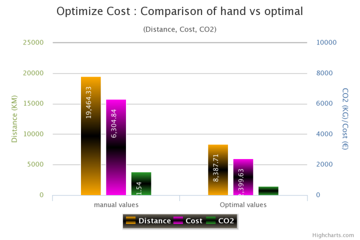
OPTIMAL	DISTANCE	9	DRIVING	7885.77 KM	88h16min35sec	2655.17 €	590.23 KG
OPTIMAL	COST	9	DRIVING	8382.39 KM	94h12min7sec	2581.36 €	608.92 KG
OPTIMAL	CO2	9	DRIVING	7938.63 KM	92h18min30sec	3227.9 €	561.33 KG
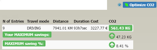
Your MAXIMUM savings:				496.61 KM	5h55min32sec	646.54 €	47.59 KG
MAXIMUM saving %:				6.3 %	6.71 %	25.05 %	8.48 %

GRAPH:

The corresponding column comparison graph will be as follows:

WHAT IS YOUR GOAL?

In this section you will get extracted summary matrix summary corresponding to your goal as indicated below for our driven example: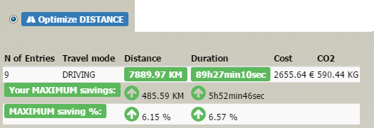

WHAT IS THE BEST AMONG THE 3 GOALS?

This step may be called only if the you want to get the best among the 3 goals only in case of different resulting matrix by goal. Otherwise, if the 3 goals have the same resulting matrix, this step is unecessary, since the 3 goals will have the same score. Getting the best of the goals uses known TOPSIS method and it gives you two options:

• Fix weight for each criterion as indicated below:
  
• No weights are affected to criteria (distance, cost, CO2) as indicated below:
  

Once you have chosen to affect or not weights, to get the the 3 goals order click on the command:
Show rank resulting matrix
You get the corresponding matrix ranking the 3 goals:
Step: Ranking result Matrix

Optmization Goal	Weights (%)	Proximity factor	Rank	Breakdown Rank (%)
Distance	30 %	0.8616491241818178	1	46 %
Cost	50 %	0.8250975846083349	2	45 %
CO2	20 %	0.16655636379250524	3	9 %

With the associated weights, distance goal is ranked 1st, cost goal is ranked 2nd and CO2 goal is ranked 3rd.

On the other hand, if the 3 criteria (distance, cost and CO2) are not weighted, you get the following matrix (which does not change ranking order with respect to the previous weighted case):

Step: Ranking result Matrix

Optmization Goal	Weights (%)	Proximity factor	Rank	Breakdown Rank (%)
Distance	100 %	0.7916213261696208	1	44 %
Cost	100 %	0.6942811923813814	2	39 %
CO2	100 %	0.29782890261426426	3	17 %

A corresponding column graph is generated and all simulated scenarios are saved in a history space as indicated below for our driven example with 2 scenarios:

Complete sample of driven examples

In order to see SMARTASS in action working dynamically for any change, try to add 1 departure point and 1 destination point as:

• 1 Departure point: add "Warsaw" as a new address. You can associate a contact to this address and change its associated "unit energy cost" and "unit CO2 emission".
• 1 Destination point: add "Frankfurt" as a new address. You can associate a contact to this address and change its associated "unit energy cost" and "unit CO2 emission".

Check all 10 deparature as well as destination points to get matrices of 10x10 dimension. Then proceed as in the 3 previous driven examples and examine that the resulting assignment matrices are diffetent. The new added 2 points will be not nessessarily associated in the matrices entries.